Examples
Getting Started
Here, we’ll find the number and times at which an object should have been scanned in Gaia DR2. Here wel will use the Source object, which has both a SkyCoord attribute giving the position and a Photometry attribute giving the photometric measurements but SkyCoord objects may also be directly applied. We specify coordinates on the sky using astropy.coordinates.SkyCoord objects. This allows us a great deal of flexibility in how we specify sky coordinates. We can use different coordinate frames (e.g., Galactic, equatorial, ecliptic), different units (e.g., degrees, radians, hour angles), and either scalar or vector input.
For our first example, let’s load the Boubert & Everall (2020, submitted) – or “cog_i” – scanning law for Gaia DR2, and then query the scanning law at one location on the sky:
from scanninglaw.source import Source
import scanninglaw.cog_i as cog_i

coords = Source('12h30m25.3s', '15d15m58.1s', frame='icrs')
scl = cog_i.dr2_sl(version='cogi_2020')
scans = scl(coords)

print('Number of scans in: FoV1={0}, FoV2={1}'.format(scans['nscan_fov1'][0], scans['nscan_fov2'][0]))
print('Scan times FoV1: {0}'.format(scans['tgaia_fov1'][0]))
print('Scan times FoV2: {0}'.format(scans['tgaia_fov2'][0]))

>>> Number of scans in: FoV1=12, FoV2=12
>>> Scan times FoV1: [1680.23593481 1680.48609923 1680.73626385 1848.39215369 1860.39690153
                      1954.98466927 2005.96485791 2139.23302501 2139.48318825 2155.73806056
                      2188.46881338 2329.27861926]
>>> Scan times FoV2: [1680.30994177 1680.56010625 1680.81027093 1812.99456365 1848.4661605
                      1860.22074468 1955.05867577 1969.81323539 2006.03886423 2139.30703225
                      2155.81206778 2188.54281976]
A couple of things to note here:
Above, we used the ICRS coordinate system, by specifying
frame=’icrs’.The output is in Gaia onboard time (in Julian Days)
Querying Scanning Law at an Array of Coordinates
We can also query an array of coordinates, as follows:
import numpy as np
from scanninglaw.source import Source
from scanninglaw import cog_i

l = np.array([0., 90., 180.])
b = np.array([15., 0., -15.])

coords = Source(l, b, unit='deg', frame='galactic')

scl = cog_i.dr2_sl(version='cogi_2020')
scl(coords)
>>> {'nscan_fov1': [18, 22, 18],
     'nscan_fov2': [18, 20, 17],
     'shape': (3,),
     'tgaia_fov1': [array([1745.60679263, 1910.87024734, ..., 2299.91611197]),
                    array([1666.54874734, 1666.79891188, ..., 2308.11154598]),
                    array([1712.59906593, 1745.73187474, ..., 2299.79102879])],
     'tgaia_fov2': [array([1712.54799105, 1745.68079934, ..., 2299.73995341]),
                    array([1666.62275438, 1666.87291882, ..., 2307.93538875]),
                    array([1712.67307241, 1745.55571791, ..., 2299.86503624])]}
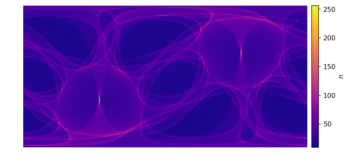
Plotting the Scanning Law
We’ll finish by plotting the distribution of number of scans in Gaia DR2 across the sky. First, we’ll import the necessary modules:
import matplotlib
import matplotlib.pyplot as plt
import numpy as np

import astropy.units as units

from scanninglaw.source import Source
from scanninglaw import cog_i
Next, we’ll set up a grid of coordinates to plot:
import astropy.units as units

l = np.linspace(-180.0, 180.0, 500)
b = np.linspace(-90.0,90.0, 250)
l, b = np.meshgrid(l, b)
g = 21.0*np.ones(l.shape)
coords = Source(l*units.deg, b*units.deg, frame='galactic')
Then, we’ll load up and query the Gaia DR2 scanning law:
scl = cog_i.dr2_sl(version='cogi_2020')
scantimes = scl(coords)
Finally, we create the figure using matplotlib:
fig = plt.figure(figsize=(12,4), dpi=150)

nscan = np.array(scantimes['nscan_fov1']).reshape(scantimes['shape'])+\
        np.array(scantimes['nscan_fov2']).reshape(scantimes['shape'])
plt.imshow(nscan,
        origin='lower',
        interpolation='nearest',
        cmap='plasma', aspect='equal',
        extent=[-180,180,-90,90])
cbar = plt.colorbar(pad=0.01)
cbar.set_label(r'$n$')


plt.axis('off')
plt.savefig('map.png', bbox_inches='tight', dpi=150)
Here’s the result: